remotes::install_github('jbryer/VisualStats')Plotting Distributions in R
R
Function and Shiny application for working with distributions in R.
When working with distributions in R, each distribution has four functions, namely:
dXXX- density function.rXXX- generate random number from this distribution.pXXX- returns the area to the left of the given value.qXXX- returns the quantile for the given value/area.
Where XXX is the distribution name (e.g. norm, binom, t, etc.).
The VisualStats::plot_distributions() function will generate four plots representing the four R distribution functions. For each subplot points correspond to the first parameter of the corresponding function (note the subplot for the random rXXX function does not have points since this simply returns random values from that distribution). The arrows correspond to what that function will return.
library(VisualStats)
data('distributions', package = 'VisualStats')
plot_distributions(dist = 'norm',
                   xvals = c(-1, 0, 0.5),
                   xmin = -4,
                   xmax = 4)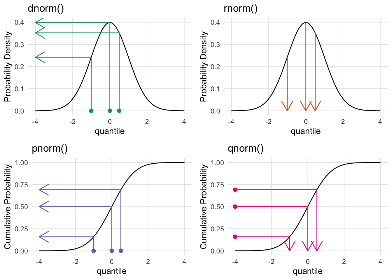
The top two plots (dXXX and rXXX) plot the distribution. The bottom two plots are the cumulative density function for the given distribution. The CDF describes the probability that a random variable (X) will be less than or equal to a specific value (x), written as F(x) = P(X ≤ x). The CDF provides a complete view of a random variable’s distribution by accumulating probabilities up to that point.
plot_distributions(dist = 'binom',
                   xvals = c(1, 3),
                   xmin = 0,
                   xmax = 10,
                   args = list(size = 10, prob = 0.35))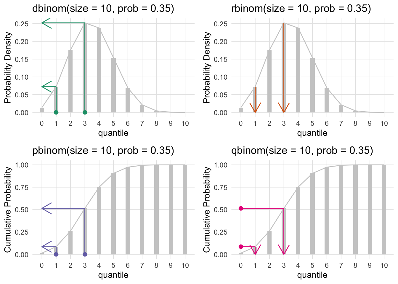
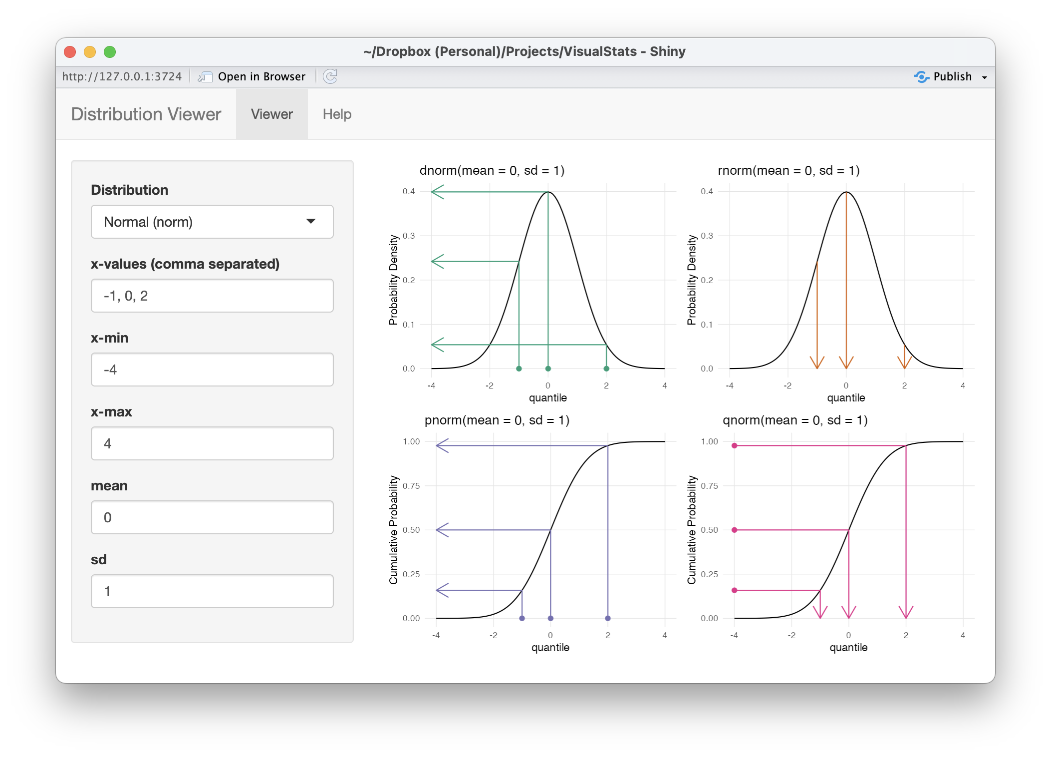
The VisualStats package also has a Shiny application that allows you to interactively plot the 17 distributions available in base R.