Why you should not use mean imputation for missing data

I encountered the question today of what to do with missing values when conducting null hypothesis testing or regression? I have seen many suggest doing mean imputation. That is, simply replace any missing values with the mean of the variable calculated from the observed values. I argue that mean imputation is worse than doing nothing. Let’s explore.

To begin, let’s simulate a vector, x, from the random normal distribution.

set.seed(2112)
x <- rnorm(100, mean = 0, sd = 1)
(mean1 <- mean(x))

[1] 0.01129628

(sd1 <- sd(x))

[1] 1.032159

We can see that the mean and standard deviation aver fairly close to 0 and 1, respectively. In the next code chunk we are going to randomly select 20% of observations and set the value to NA. We can calculate the mean and standard deviation excluding the missing values (i.e. NAs) but setting na.rm = TRUE. The mean and standard deviation are relatively close.

x[sample(length(x), length(x) * 0.2, replace = FALSE)] <- NA
(mean2 <- mean(x, na.rm = TRUE))

[1] 0.02136184

(sd2 <- sd(x, na.rm = TRUE))

[1] 1.071757

Now we will replace the NAs we introduced above with the mean. We can see that the standard deviation is quite a bit smaller, hence reducing the variance of our estimate. Since many of our statistical tests rely on variance, reducing the variance may lead to spurious conclusions.

x[is.na(x)] <- mean(x, na.rm = TRUE)
(mean3 <- mean(x))

[1] 0.02136184

(sd3 <- sd(x))

[1] 0.9573977

To show this is not a random anomaly for our one random sample, let’s repeat the above 1,000 times.

n_samples <- 1000
percent_missing <- 0.10
sd_diffs <- data.frame(sample = 1:n_samples,
                       sd_drop_miss = numeric(n_samples),
                       sd_impute_miss = numeric(n_samples))
for(i in seq_len(n_samples)) {
    x2 <- x
    x2[sample(length(x), length(x) * percent_missing, replace = FALSE)] <- NA
    sd_diffs[i,]$sd_drop_miss <- sd(x2, na.rm = TRUE)
    x2[is.na(x2)] <- mean(x2, na.rm = TRUE)
    sd_diffs[i,]$sd_impute_miss <- sd(x2)
}

sd_diffs |> 
    reshape2::melt(id.vars = 'sample', variable.name = 'calculation_type', value.name = 'sd') |>
    ggplot(aes(x = sd, color = calculation_type)) +
        geom_vline(xintercept = sd(x)) +
        geom_density() +
        xlab('Standard Deviation') +
        theme_minimal()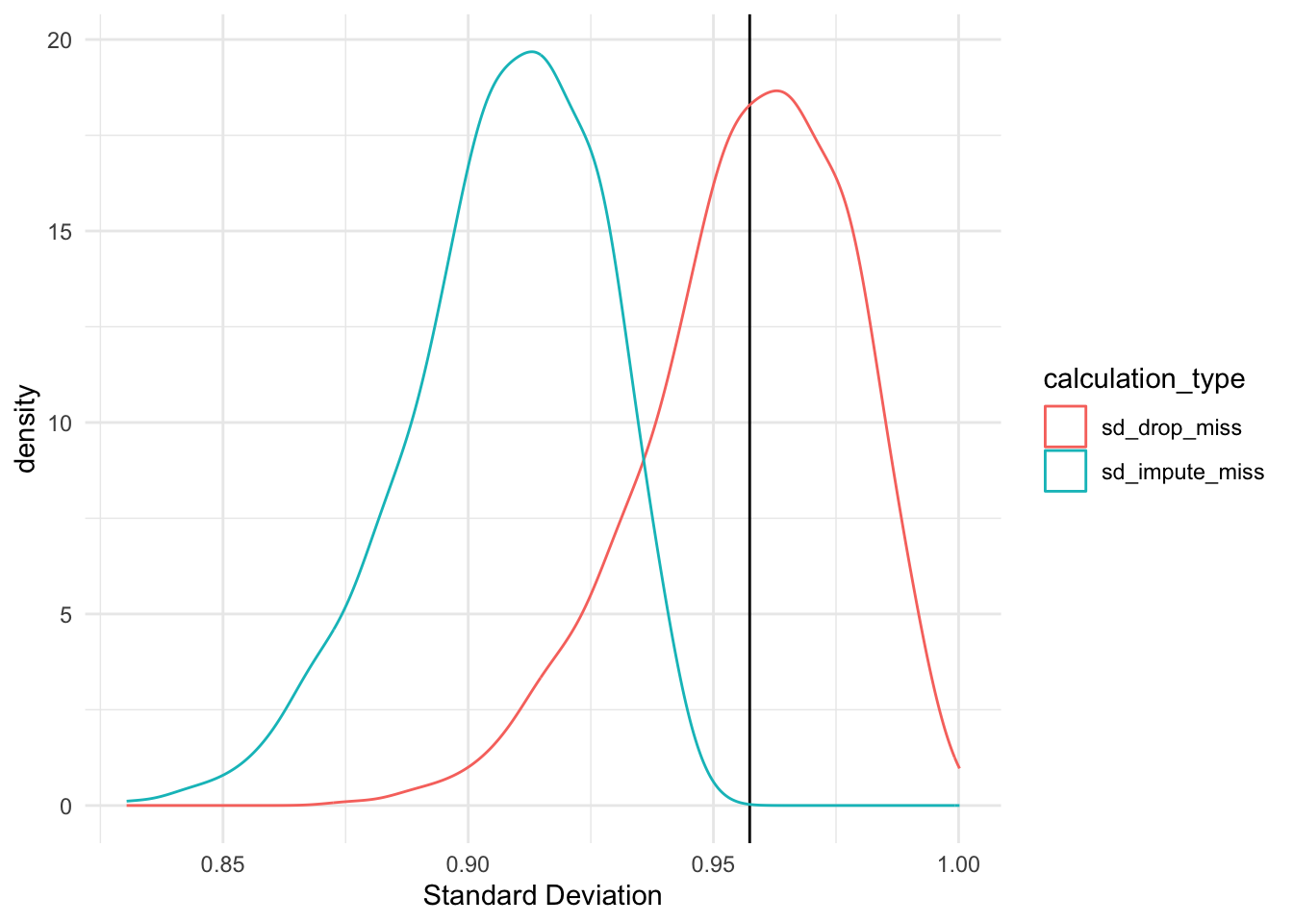

As the figure above shows, there is a significant difference in the standard deviation estimates when calculated using only observed values and calculated with missing values imputed with the mean. The t-test below confirms this.

t.test(sd_diffs$sd_drop_miss, sd_diffs$sd_impute_miss)

    Welch Two Sample t-test

data:  sd_diffs$sd_drop_miss and sd_diffs$sd_impute_miss
t = 54.288, df = 1992.4, p-value < 2.2e-16
alternative hypothesis: true difference in means is not equal to 0
95 percent confidence interval:
 0.04782442 0.05140925
sample estimates:
mean of x mean of y 
0.9569447 0.9073278 

Now let’s consider how mean imputation can impact the estimation of a correlation between two variables. We will simulate two variables with a population correlation of 0.18.

n <- 100
mean_x <- 0
mean_y <- 0
sd_x <- 1
sd_y <- 1
rho <- 0.18

set.seed(2112)
df <- mvtnorm::rmvnorm(
    n = 100,
    mean = c(mean_x, mean_y),
    sigma = matrix(c(sd_x^2, rho * (sd_x * sd_y),
                     rho * (sd_x * sd_y), sd_y^2), 2, 2)) |>
    as.data.frame() |>
    dplyr::rename(x = V1, y = V2)

cor.test(df$x, df$y)

    Pearson's product-moment correlation

data:  df$x and df$y
t = 1.8314, df = 98, p-value = 0.07008
alternative hypothesis: true correlation is not equal to 0
95 percent confidence interval:
 -0.01504323  0.36527878
sample estimates:
      cor 
0.1819124 

We will now randomly select 20% of x values to set to NA.

df_miss <- df
df_miss[sample(n, size = 0.2 * n, replace = FALSE),]$x <- NA
cor.test(df_miss$x, df_miss$y)

    Pearson's product-moment correlation

data:  df_miss$x and df_miss$y
t = 1.8392, df = 78, p-value = 0.06969
alternative hypothesis: true correlation is not equal to 0
95 percent confidence interval:
 -0.01658176  0.40543327
sample estimates:
      cor 
0.2038779 

Note that the p-value for both the correlation estimated using the complete dataset and estimated with observed values only is greater than 0.05 (i.e. we would fail to reject the null that the correlation is 0).

Now we will impute the missing values with the mean and calcualte the correlation.

df_miss[is.na(df_miss$x),] <- mean(df$x, na.rm = TRUE)
cor.test(df_miss$x, df_miss$y)

    Pearson's product-moment correlation

data:  df_miss$x and df_miss$y
t = 2.0582, df = 98, p-value = 0.04223
alternative hypothesis: true correlation is not equal to 0
95 percent confidence interval:
 0.007431517 0.384594022
sample estimates:
      cor 
0.2035525 

We would now reject the null and conclude that there is a statistically significant correlation between x and y even though our original dataset from which this was simulated was not.